Tensors
Here is the first part of a series of courses of initiation to
tensors.
What are tensors ? Beyond the definition of that notion, the study
of tensors forms a theory with its own mathematical
framework, namely a formal grammar expressing linear algebra
better than by ordinary algebraic terms.
Why tensors ? The main motivation is its indispensability to express
modern physics (General Relativity and
quantum physics) and even its usefulness to greatly clarify the
expression of classical physics (conservation
laws in classical or relativistic mechanics, electromagnetism) which
looks awful without it.
Unfortunately, usual courses of classical physics keep their old
awkward formulations, missing the clarifications that tensors could
provide, due to the bad reputation of tensors as a hard,
inaccessible or messy topic to be reserved for a later year of
teaching. Actually, this trouble relies on the way tensors are
usually introduced, which I consider inappropriate, and could
hopefully vanish by adopting a different approach. So, I will
provide here my view on the topic in try to make it clearer and
easier to learn.
I usually only make courses in text form, which is easier for me to
work on. This would not suffice here because of geometrical aspects
which need to be visualized. But I'm still more at ease writing than
speaking. So I made here both text and video formats, which will be
meant as complementary : some things will be only in video, others
only in text.
1. Reminder on vector spaces and linear algebra.
A vector space is a set E with structures (operations)
- 0 (constant)
- + (addition) : E×E → E
- . ("multiplication by a real number") : ℝ×E → E
(or ℝ-indexed family of functions)
satisfying the same identities as the operations with the same names
in ℝ, when expressible between these sets.
From there, subtraction can be defined as
Vector spaces appear in geometry in different ways, where the 2 most
intuitive are:
- As translations (+ is composition) : the "space of vectors"
of a given affine space;
- As a space (an affine space) with a choice of 0 : x+y
is defined by parallelogram (x, 0, y, x+y).
The latter is the most common way to imagine a vector space, which
may involve new figures separate from those we could start with.
Vector spaces are classified by their dimension : a natural number,
or infinity (the diversity of infinite dimensions does not matter
for physics, we shall ignore it here).
ℝ is a 1-dimensional vector space.
For now, vector spaces (with dimension 2 or more) are handled
without any measure of angles, or equivalently (in the sense of
mutual definability) any distinction of squares among
parallelograms, or of circles among ellipses. Vector spaces with
such additional structures, called Euclidean vector spaces, will be
discussed later.
We sometimes use complex vector spaces, replacing the role of the
system ℝ of real numbers by that ℂ of complex numbers. So, ℂ is a
2-dimensional ℝ-vector space (precisely, an Euclidean one), but
1-dimensional as a complex vector space; n-dimensional
complex spaces are 2n-dimensional in the sense of ℝ-vector
spaces (not a priori Euclidean when n>1).
Important kind of vector space : the space EX
of all functions from a set X to a vector space E.
Its structures are defined from those of E.
Its dimension is : (Card X).(dim E)
So if E = ℝ, its dimension is Card X.
Vector subspace : subset stable by all
operations (0,+,.)
Those of a 3D space E: {0}, straight lines and planes
containing 0, and E.
The subspace of a vector space E generated by a set X
⊂ E is equivalently defined as
- The smallest (for ⊂) subspace F ⊂ E such that
X ⊂ F (like any subalgebra)
- The set of all linear combinations of elements of X,
i.e. a1.x1+...+ an.xn
for any n∈ℕ and tuples a∈ℝn,
x∈Xn.
A vector space of functions from X to E : is
a vector subspace of EX.
A function f : E → F between vector spaces E,
F is linear (we shall say a linear map) if it
preserves all operations.
Then its image (Im f) is a vector subspace of F, and
its kernel
Ker f = {x∈E | f(x)
= 0}
is a vector subspace of E.
For any vector space H of functions from X to E,
any x∈X defines a linear map (f ↦ f(x))
from H to E.
The set L(E,F) of all linear maps from E to F
is a vector space of functions (vector subspace of FE),
thanks to the properties of operations. Its dimension is the product
of dimensions (dim E).(dim F).
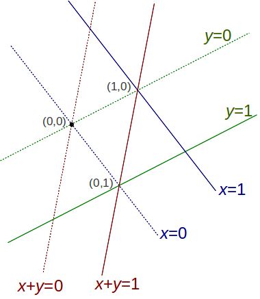
Linear maps from E to ℝ are called linear forms on E,
or covectors.
The space E* of all covectors of E is called the dual
of E.
Nonzero covectors can be visualized by their kernel (hyperplane :
dimension n−1) and its parallel space with value 1.
For any vector spaces E,F,G, an operation
(function of 2 variables) : E×F → G is called
bilinear if linear on each variable when the other is fixed,
i.e. one curried form is in L(E,
L(F,G)); equivalently the other curried form is in L(F,
L(E,G)).
The operation ⚬ of composition of linear maps, from L(F,G)×L(E,F)
to L(E,G), is bilinear. Naming elements as
f ∈ L(E,F)
g ∈ L(F,G)
g⚬f ∈ L(E,G)
the linearity on f (i.e of f ↦ g⚬f)
is because g is linear.
The linearity on g still holds when only G is a
vector space, and f is any function; there, it is deduced
from the above (with H).
If E = ℝ then L(E,F) is essentially F
(namely {(a ↦ a.x) | x∈F}),
which gives the bilinearity of the function
evaluator (g,y) ↦ g(y) from L(F,G)×F
to G.
If G = ℝ we get the linearity of transposition
from L(E,F) to L(F*,E*).
If F = ℝ we get the bilinearity of the tensor product
⊗ : G × E* → L(E,G)
This is just one of the possible definitions of the tensor
product of elements, only equivalent for finite dimensional
spaces.
But a proper understanding and formalization of tensors requires
another definition of tensor products, allowing for any number of
arguments, treated symmetrically. Here the symmetry of roles between
G and E* can appear by transposing the target space,
from L(E,G) to L(G*,E*).
But a symmetry between 2 definitions is not good. In their own
framework, tensors will have 1 symmetric definition.
To make things really clean, we need to rebuild linear algebra on a
different foundation: aside the usual definition and treatment of
vector spaces which we shall call "algebraic", let us introduce
another definition, as dual systems.
2. The category of dual systems
To provide the semantics for the tensorial formalism, linear algebra
needs to be redefined from the concept of dual systems. This fact
seems strangely unnoticed, as the big Wikipedia article on "dual
systems" currently (2022) is not linked with articles on tensors
either way, while the Wikipedia article on "dual spaces" only has
small links with key phrases "dual systems" and "dual pairs", as if
dual systems could only interest some analysis of infinite
dimensional spaces. Also the article on dual systems assumes the
background of all algebraic concepts on vector spaces, ignoring that
linear algebra can be simplified by starting with dual systems to
bypass some tedious aspects of the algebraic approach.
A dual system, or dual pair, is a pair of sets (E,E')
qualified as "dual of each other", with an operation called duality
pairing
〈 , 〉 : E×E' → ℝ.
Only needed axioms:
Each curried form of a duality pairing is injective,
with image a vector space of functions.
The injectivity of the curried form from E to E'* is
written
∀x,y∈E, (∀z∈E', 〈x,z〉
= 〈y,z〉) ⇒ x = y.
We can write ⇔ instead of ⇒ since the converse always holds (an equality
axiom).
Structures in each vector space E and E', are
defined by copying those on their images, restrictions of those on
spaces of all functions from given sets to ℝ, themselves defined
from those of ℝ ; the axioms for algebraic vector spaces are
deducible from identities in ℝ. This makes 〈 , 〉 bilinear.
We shall often identify E' with its copy as a subspace of
E*, and also symmetrically, identify E with its
copy as a subspace of E'* (letting the duality pairing
play on both sides the role of function evaluator).
Both definitions (algebraic and with duality) are equivalent for
finite dimension spaces (where the algebraic E* is the only
possible dual of E) but not otherwise : for an infinite
dimensional E, different infinite dimensional subspaces of E*
may serve as duals of E.
Even, without the Axiom of Choice, there
can exist vector spaces with no duality representative, that is when
the natural map from E to E** is not injective. In
particular the algebraic dual of an infinite dimensional space can
have dimension 0. Such spaces have no interest for physics, so we
shall ignore them.
Between dual pairs (E,E') and (F,F'), a
map f : E→F will be qualified as transposable
if
∀y∈F', ∃z∈E', ∀x∈E,
〈x,z〉 = 〈f(x),y〉
or in short
∀y∈F', y⚬f ∈E'
which means the existence of a (unique) function tf
: F'→E' called the transpose of f,
such that
∀x∈E, ∀y∈F', 〈f(x),y〉
= 〈x,tf(y)〉.
Seeing ℝ as part of the dual pair (ℝ,ℝ) with duality pairing given
by multiplication, the condition for a y∈ℝE
to be transposable from (E,E') to (ℝ,ℝ) is that
y∈E' ; the transpose is then (a ↦ a.y).
Transposability implies linearity, and thus both properties are
equivalent in finite dimensional cases.
In infinite dimensions, there is a concept of topological vector
spaces, with continuous linear maps. For a certain topology, this
condition of linearity+continuity coincides with transposability.
Let us forget this and directly work with the simplest concept, that
is the transposability of maps between dual systems.
Since the use of transposability will replace for us linearity,
while the word "linearity" is much more familiar and equivalent to
transposability for our main purpose (finite dimensional spaces),
let us decide that from now on, we shall use the word "linearity" to
actually mean transposability when used between spaces with given
choices of duals. Similarly, the "bilinearity" of a binary operation
will implicitly mean the transposability of the function it defines
when either argument is fixed, if a dual is indeed given for the
domain and target spaces of that function.
Dual pairs form a category, where morphisms from (E,E')
to (F,F') are pairs of maps (f,f')
where f : E→F and f': F'→E'
are the transpose of each other.
In other words, f and f' play the roles of both
curried forms of the same operation from E×F'
to ℝ, where duality pairings play the role of function evaluator on
both sides.
Compared to the usual function evaluator written y(x)
for x∈E and y ∈ ℝE, the use
of the pairing 〈x,y〉 requires that moreover,
essentially, y belongs to the subspace E' of
ℝE.
This operation E×F'∋(x,y) ↦ 〈f(x),y〉
is bilinear. Actually, the bilinearity of an operation from E×F'
to ℝ is equivalent to the existence of such curried forms for it on
both sides, thus transpose of each other and forming a morphism in
this category.
Now the concept of tensor comes by considering that these 3 things :
- A linear map f : E→F
- Its transpose f': F'→E'
- A bilinear operation from E×F' to ℝ
being definable from each other, need to be seen as just 3 different
roles of one same thing, called a tensor of order 2 with
type (E', F), element of what we shall call the complete
tensor product
E'⊠F (which assumes the implicit data of the dual
system which each space is seen a member of).
With conventions E'⊂ℝE and F'⊂ℝF,
this definition for E'⊠F' (picking now F'
instead of F) can also be written using the sum of functions ∐ as:
E'⊠F' = {∐f | f∈F'E}
⋂ {t∐g | g∈E'F}
= {h∈ℝE×F| (Im h⃗
⊂ F') ∧ (Im h⃖ ⊂ E')}
3. Tensor notations
To work in practice with this concept of tensors of order n
with their n+1 (or even more) different but equivalent uses
as operations (which usual courses of linear algebra keep
unfortunately distinguishing), we need to replace the notations we
were using by a different notations system, that is the tensorial
notations. Let us start with some definitions.
Generally, we shall call tensor any element of a vector
space (which belongs to some dual system), and the type of a
tensor is a way of naming this vector space it is seen an element
of.
The order of a tensor, determined by its type, essentially
means its arity, precisely the arity it takes as an operation with
values in either ℝ or another 1-dimensional space (kind of
quantity). Any tensor of order n, seen as an n-ary
operation, must be n-linear (we shall say multilinear
to not specify n), which means linear with respect to each
of its arguments when others are fixed. So, the above tensor was
said to be of order 2 because of its role as a bilinear operation
with values in ℝ, but also because no further context was given for
this construction. Actually the order attribute we give to vector
spaces may depend on context.
All vector spaces which were given as primitive, and their duals,
are said to be of order 1, except for ℝ and other 1-dimensional
spaces, which are said to be of order 0 for reasons which will be
clear later.
Just like operation symbols are symbols with n places for
its arguments around, and families being synonyms for functions
(unary operations) display their argument as an index, now a tensor
of order n will be denoted as a symbol with places for n
attached indices, which represent its arguments, although
the arguments we may effectively give for it will not be written
there.
Among the terms admitted in the tensor formalism, the monomial
ones are those not using + or −, and therefore multilinear with
respect to all occurrences of tensor symbols inside. The structure
of these monomial terms will be expressed by the positions of
index symbols attached to each tensor symbol, while the writing
order between tensor symbols will be irrelevant.
So, given a dual pair (E,E'),
- Any element y ∈ E' gets a notation of the
form yi where the chosen index symbol i
refers to the argument in E which y depends on
for giving value in ℝ ;
- Any element x ∈ E gets a similar notation,
either of the same form xi, or the form xi
(with an upper index) in formal contexts where, for any reason,
a visible distinction of roles between "vectors" and "covectors"
will be needed;
- The duality pairing between some x ∈ E, y
∈ E' will be written by letting them in any order but
with a repetition of the same index, to mean they are applied to
each other :
xi yi = xk
yk = yi xi
= 〈x,y〉
Repeated indices in a monomial are "internal to this monomial" and
may be so renamed inside it without affecting its meaning.
Non-repeated indices matter as they represent the type of the value
of this monomial as a tensor, and so must be repeated between
monomials separated in the same equation by +, − , = ; they may only
be globally renamed there.
The same tensorial formalism we are introducing, can be pictured by
another notations system called the tensor diagram notation:
monomial terms are figured as diagrams where
- a symbol of tensor with order n serves as a vertex
with n branches, more precisely a "small box" with n
"plugs for edges".
- A repeated index becomes an edge connecting its two
occurrences
- A non-repeated index becomes an edge connecting its occurrence
to "the plug marked by this index" at the "border of the big
box" which contains the diagram.
Actually in particle physics, Feynman diagrams need to be read
as tensorial expressions in this way.
Now any tensor of order 2 (binary tensor) will be written with 2
indices. To take the same names as above, a binary tensor T
∈ E'⊠F, relating given dual pairs (E,E')
and (F,F'), can be written Tij
where
- i refers to its E'-ness (dependence on
an argument in E);
- j refers to its F-ness (dependence on an
argument in F');
- The role of T as a map f : E→F
is written ∀x∈E, ∀z∈F, z = f(x)
⇔ zj = Tij
xi
- Its transpose f': F'→E' is
written ∀y∈F', ∀u∈E', u = f'(y)
⇔ ui = Tij
yj
The axiom making them the transpose of each other is written
∀x∈E, ∀y∈F', (Tij
xi) yj = xi
(Tij yj)
This means that parenthesis are useless in monomials; they will be
dropped there and only still used to contain both + and −
operations, and also specify the scope of the differentiation symbol
∂.
Any dual pair (E,E') has a Kronecker delta
symbol δ ∈ E'⊠E serving as the duality
pairing of (E,E'), and equivalently as the
identity function in each of E,E':
∀x∈E, δij
xi = xj
∀y∈E', δij
yj = yi
∀x∈E,∀y∈E', δij
xi yj = xj
yj = xi yi
Elements of 1-dimensional spaces, called quantities, are
seen as of order 0 because they do not need an index in monomials,
as they can be multiplied in any order, and tensors can be
multiplied by them with the same rules in monomials as with real
numbers. The only difference this makes from real numbers is the
different 1-dimensional target space (instead of ℝ) of tensors and
tensorial expressions as multilinear operations (it needs to be
the same between monomials in an equation).
I had to introduce this definition and notation ⊠ for
convenience, away from the tradition of only defining the tensor
product ⊗ of vector spaces independently of their duals.
Another text will give the definition of the tensor product,
with technical justifications for some aspects of the formalism we
just developed, especially
- how, for any dual pairs (E,E') and (F,F'),
the space E⊠F forms a dual pair with the tensor
product space E'⊗F' which has a bilinear form ⊗ :
E'×F' → E'⊗F' such that ∀T∈
E⊠F, ∀x∈E',∀y∈F', 〈T,
x⊗y〉 = Tij xi
yj.
- how moreover E⊗F ⊂ E⊠F, with
equality when any of E or F is finite
dimensional.
- the definition of the trace of any T∈ E'⊗E,
that is Tii = 〈T,δ〉
- why the dimension of any vector space equals the trace δii
of its Kronecker delta (which also explains we cannot take this
trace for infinite dimensional spaces, i.e. δ ∈ E'⊠E
\ E'⊗E).
4. Symmetry and antisymmetry
A tensor with all arguments in the same space is called
- symmetric if it is unchanged by any permutation of
these arguments.
- antisymmetric if unchanged by even
permutations, but turns to its opposite by any odd
permutations such as transpositions.
For a tensor T with order 2, it is symmetric if Tij
=Tji, and antisymmetric if Tij
= -Tji.
The spaces of symmetric tensors, and antisymmetric tensors, of
order n in E (subspaces of ⊠n E
= E ⊠ ... ⊠ E), are respectively
denoted Symn E and
Λn E.
As any involutive linear transformation is a reflection,
the transposition of indices is a reflection in respect to the
subspace of symmetric tensors, in parallel to that of antisymmetric
ones.
Like any reflection, it can be used to express both linear
projections, over each of these two subspaces in parallel to the
other.
So, any tensor T ∈ E⊠E has a unique
expression as a sum T = S + A where S is
symmetric and A is antisymmetric, namely
Sij = (1/2).(Tij
+ Tji)
Aij = (1/2).(Tij − Tji)
The dimensions of both subspaces Sym2E and Λ2E
can then be calculated as the traces of these projections to each (T
↦ S and T ↦ A), namely (with n = dim
E)
dim Sym2E = n(n+1)/2
dim Λ2E = n(n−1)/2
Quadratic forms
Any tensor T ∈ E'⊠E' (bilinear form on E)
defines a quadratic form Q = (E ∋ x ↦
T(x,x)). The kernel of this linear map (T↦Q)
: E'⊠E' → ℝE is Λ2 E',
(why)
so that quadratic forms are actually presentations of symmetric
tensors S ∈ Sym2 E.
Indeed we can restore S from Q as
∀x,y∈E, 2 S(x,y)
= Q(x+y) − Q(x) − Q(y).
A more interesting formula uses the differential of Q as a
field : the covector ∂jQ(x) is
defined as ∂jQ(x) yj
being an approximation of Q(x+y) − Q(x)
for any small y. When y is small, Q(y)
is neglected. So, the previous formula gives by approximation
∀x∈E, 2 Sij xi
= ∂jQ(x)
The most often used symmetric bilinear forms are those whose
quadratic form is positive on nonzero vectors : synonymously called
"dot products" or "inner products" (in French there is only one
name, "produit scalaire"). This is the fundamental structure giving
an Euclidean geometry to a vector space. For this to describe the
vectors of the usual physical space which has no most favorite unit
of distance, its values are quantities (squared lengths).
The dot product in an Euclidean plane E (correspondence with
its dual) can be understood by 3D drawings : either
Self-duality
If a tensor T ∈ E'⊠E' is invertible (also
called "non-degenerate"), then T -1 ∈ E⊠E,
and with the same property of symmetry or antisymmetry as T.
Giving such a T as a structure on E, can be
formalized by declaring E to be self-dual, and using T
as duality pairing. This is done only when T is either
symmetric or antisymmetric (otherwise its symmetric and
antisymmetric components would be 2 structures to distinguish on
that space): a self-dual vector space is either qualified as
- Quadratic if its duality pairing is symmetric
- Symplectic if its duality pairing is antisymmetric.
Unfortunately, this is usually done too often in usual teaching, so
that people keep inappropriately defining as vectors what should
rather be seen as covectors, to the point that they may have no clue
what a covector is (unless they don't even know what a vector is
either, as they only work with arrays of numbers serving as
coordinates of anything, forgetting that, well, Nature does not fix
a favorite choice of coordinates system in physical space). This can
become a handicap as it binds them to Euclidean geometry and makes
it harder for them to learn different geometries. And no, physical
space is actually not Euclidean.
Any 2-dimensional vector space is symplectic.
The dimension of a symplectic space is always even.
In a 2D Euclidean space (plane), composing its quadratic and
symplectic structures gives its complex structure (multiplication by
i).
5. Orthogonality
In a finite dimensional Euclidean vector space E, 2
vectors x,y are said to be orthogonal if 〈x,y〉
= 0.
This defines a Galois
connection, which is symmetric : (⊥,⊥) ∈
Gal(℘(E),
℘(E)).
The closed elements of this connection are the vector subspaces.
The closure of a set is the vector subspace it generates.
If E has dimension n and a subspace F ⊂ E
has dimension k then ⊥F has dimension n−k
because a basis of F and a basis of ⊥F together
form a basis of E.
Now these definitions do not really need the space to be
Euclidean, except for the argument with basis, which needs to be
replaced.
For any dual pair (E,E'), orthogonality defines in
the same way
a Galois connection (⊥,⊤) ∈ Gal(℘(E),℘(E')).
Again on each side, closed elements are the vector subspaces.
Except that, infinite dimensional subspaces are not always closed.
So, the study of infinite dimensional dual pairs requires to speak
about closed subspaces, which are a special kind of vector
subspace. We shall not really care about this, but will still
write general definitions in ways still valid then.
Now, in the usual visualization of an n-dimensional
vector space E as a set of points, a k-dimensional
subspace H of E' can be visualized by means of
its orthogonal, that is an (n−k)-dimensional
subspace F of E.
Namely H can be seen as a dual of the quotient space E/F.
Drawing of quotient in https://spoirier.lautre.net/no12.pdf
page 8.
In any dual pair (E,E'), any subspace F ⊂ E
naturally gets a dual F' = tIdF
[E'] making IdF an embedding
from (F,F') to (E,E').
Here, Ker tIdF = ⊥F.
Then (tIdF is a quotient
from (E',E) to (F',F))
⇔ (F is closed).
Any binary tensor T = (f, f') ∈ E⊠F
where f : E'→F and f': F'→E
has a left image Im f' ⊂ E and a right image Im f
⊂ F.
It also has a left kernel Ker f = ⊥Im f' ⊂ E'
and a right kernel Ker f'= ⊥Im f ⊂ F',
which are closed subspaces.
As well-known in linear algebra, the equivalence
relation ∼f of any linear map f is
expressible from Ker f as
x ∼f y ⇔ x
− y ∈ Ker f
Generally, from any subspace A ⊂ E, we can define an
equivalence relation this way (x ∼ y ⇔ x − y
∈ A), making the quotient E/A a vector space.
However, for this quotient to be part of a dual system making
transposable the surjection ϕ: E
↠ E/A we need A to be closed. Then its
transpose is injective, ϕ' : (E/A)' ↪ ⊥A and ⊥A
is the closure of Im ϕ'. Now to make ϕ a quotient we must take ⊥A
as dual of E/A, letting this construction coincide
with the above one for the embedding of ⊥A into E'.
There is only the inessential difference that we now define the
quotient as proceeding by an equivalence relation, while it was
previously defined by restricting covectors, seen as functions, on a
subspace. To make things explicit, the duality pairing on (E/A,
⊥A) can be defined by
∀x∈E,∀x∈⊥A, 〈ϕ(x),y〉
= 〈x,y〉.
Similarly, any binary tensor T = (f, f') ∈ E⊠F
defines a pairing between its left image Im f' ↔ F'/Ker
f' and its right image Im f ↔ E'/Ker f
. Thus, these 4 spaces have the same dimension, which is called the
rank of T.
Antisymmetrization
The p-antisymmetrizer, officially
called the generalized Kronecker
delta of order 2p over a given dual pair (E,E'),
has p upper indices and p lower indices. It
"provides antisymmetry" over p indices, may they be all up
or all down, by summing up all diagrams expressing the p!
permutations of these indices, with sign given by the signatures
of these permutations. Thus, it maps any tensor of order p
to its antisymmetric component multiplied by p!.
For example with p = 2,
δijkl
= δik δjl
− δil δjk
Given a dual pair (E,E') with
dimension n, the space Λn E' is
1-dimensional, represented by a generating element εijk...
we shall call a/the lower Levi-Civita symbol of E. This
tensor gives the determinant of any n-tuple of vectors in
E, i.e. the volume of the parallelepiped they form, with
sign expressing their orientation.
(Why : drawings 2D, 3D..)
It can be seen as an antisymmetric n-linear map from En
to a copy of Λn E seen as a separate
1-dimensional space, namely the vector line of quantities "volumes
in E signed by the orientation". The space E is said
to be oriented if qualifications of "positive" vs "negative"
are given to both sides of this line. Any choice of lower
Levi-Civita symbol of E, namely a choice of a favorite or no
favorite unit of volume, and a choice of orientation or no
orientation, determines the convention for its "inverse" : the upper
Levi-Civita εijk... symbol of E,
generator of Λn E, playing a symmetric
role by duality. Namely, when seen as an n-linear form on E',
it takes value in a copy of Λn E always
considered as "the inverse line" to Λn E'.
Namely, this inversion rule, to define "the same unit of volume"
and "the same orientation", is such that their product gives the
antisymmetrizer: for example
εij εkl
= δijkl
Representing subspaces by antisymmetric tensors
Any k-dimensional subspace A ⊂ E, can be
given in the form of its upper Levi-Civita symbol, i.e. a generator
of Λk A ⊂ Λk E.
It can be obtained by applying the antisymmetrizer to a basis of k
elements of A (which gives it the volume of this basis). For
example with k=2, and a basis (a,b) of A,
this is written a∧b. In index
notations,
(a∧b)kl= δijkl
ai bj = ak
bl − al bk
Now the (n−k)-dimensional subspace ⊥A of E'
where n = dim E, is similarly expressible by its
Levi-Civita symbol, generator of Λn−k
⊥A ⊂ Λn−k
E', which can also be written from a basis of A using
the lower Levi-Civita symbol of E. Namely with k=2
and n=5, and a basis (a,b) of A,
εijklm ai
bj
6. Review of quadratic spaces
In the same way, other kinds of bilinear
forms give other geometries. Unfortunately, usual courses do not
have a name for these other structures, as if they were not real,
though our actual physical space is not Euclidean. Because it is
4D, described by the Minkowski geometry, which differs from
Euclidean geometry by the fact the scalar square of its vectors is
not positive. According to Wikipedia,
where it is described, "The Minkowski inner product is not an
inner product", and "It is also called the relativistic dot
product".
Quadratic forms 2D are represented by paraboloids.
(google images)
- Elliptic paraboloids : Euclidean
geometry, may differ from the one used to visualize the space
before introducing a quadratic form there. Horizontal sections
("circles") are ellipses centered on 0 (while other plane
sections are circles with different centers)
- Hyperbolic paraboloid. Horizontal
sections ("circles") are hyperbolas.
- In between : degenerate.
Wikipedia :
Paraboloid : image
of elliptic paraboloid, parabolic cylinder, hyperbolic paraboloid
Quadratic forms 3D appear by "their
spheres" which are quadrics
Illustrations(12.6.13).
Geometric description of orthogonality of subspaces with respect
to a cone.
For any quadratic form (with bilinear
form b), its signature is a pair (p,q) where
- p is the maximum dimension of Euclidean subspaces i.e.
nonzero vectors have positive scalar squares.
- q is the maximum dimension of negative Euclidean
subspaces (scalar squares are negative)
Then the rank of b is p+q. Thus p+q
= n if b is non-degenerate in an n-dimensional
space.
Essentially, signatures (p,q) and (q,p)
are synonymous, describing the same geometry, since they are
exchanged when replacing b by -b.
A subspace A ⊂ E of a quadratic space, is called
regular if A ∩ ⊥A = {0}.
Equivalently, the restriction to A of the inner product of
E is non-degenerate, making A a quadratic space.
The symplectic structure of a 2-dim space E
gives an isomorphism between E and E', thus
between E⊠E and E'⊠E', and between
Sym2 E and its dual Sym2 E'.
This makes Sym2 E a quadratic space with
signature (1,2).
Illustration.
Correspondence between directions in E
and directions in the cone (symmetric squares of vectors).
The null directions of a quadratic form (b ∈ Sym2
E) in E are those of the intersection of ⊥b
with the cone.
Illustration of the symmetric product of 2 vectors : orthogonal
to both vectors
...
The symplectic structures of two 2-dim
spaces E, F give an isomorphism between E⊠F
and E'⊠F'. This makes E⊠F a
quadratic space with signature (2,2).
Its null vectors are the rank 1 tensors.
Illustration by using the previous representation (E = F),
3D + the 4th dimension representing the antisymmetric part.
Illustration in projective form : the cone appears, depending on
the choice of projective representation, either as an hyperbolic
paraboloid, or as a hyperboloid.
In each case, we notice a grid of straight lines, which correspond
to the x⊗y for fixed x and variable y,
or vice versa. The view as an hyperboloid corresponds to the view
(E = F) as the subspace of symmetric tensors is
sent to infinity.
Finally, starting with a 4D space E, its Levi-Civita
symbol gives to the space Λ2E (antisymmetric
binary tensors) a quadratic structure (let us write it ε)
with signature (3,3). Its cone is made of (antisymmetric) elements
with rank 2, while other elements have rank 4; it contains 2 kinds
of 3D vector subspaces (which correspond to the duality of roles
of E and E'):
- Those made of all elements of the form a∧b
for fixed a and variable b;
- Those contained in Λ2F for some 3D subspace
F of E.
If E is also given a quadratic structure then this brings
another quadratic structure b on Λ2E
with signatures as follows
| Signature of E |
Signature of b |
(4,0) or (0,4)
|
(6,0)
|
(3,1) or (3,1)
|
(3,3)
|
(2,2)
|
(2,4)
|
Composing ε and b gives a transformation of Λ2E.
In the cases of even signatures ((4,0) or (2,2)) this
transformation is a reflection (involution), splitting Λ2E
as a sum X+Y of two quadratic 3D subspaces.
In the (2,2) case the restrictions of b to X and Y
have signature (1,2) and represent Sym2 A and
Sym2 B where E= A⊠B.
In the (4,0) case, X and Y are of course
Euclidean. This role of a 4D Euclidean space as a space of
correspondences between two 3D Euclidean spaces, appears in
particular to represent the structure of the set of all maximally
entangled states of a system of 2 qbits; it also has strong links
with the algebra of quaternions.
Giving an element i of X then amounts to giving to
E a complex structure (then a Hilbert space with 2 complex
dimensions), whose 1D complex projective space corresponds to the
sphere
of Y. Then completing i to form an orthogonal
basis (i,j,k) of X, these j,k
form the real and imaginary parts of a Levi-Civita symbol for E
as a 2D complex space.
In a Minkowski space E (signature (3,1)) this composition
of ε and b gives not a reflection but a complex
structure, making Λ2E a complex quadratic space,
with complex dimension 3, and its complex bilinear symmetric form
is b + i ε where each of b and ε
is meant in its initial sense of real bilinear form. An important
role of Λ2E is as the space of values of the
electromagnetic field at a point of space-time. A choice of
reference frame (time direction) leads to a split of its elements
as E + i B where E and B
are the "electric" and "magnetic" fields in 3D.
This 3D quadratic complex space, similarly to real quadratic
spaces with signature (1,2), can be seen as the space of symmetric
bilinear forms on a 2D complex space called the space of spinors
of space-time. Its 1D complex projective space, transformed by the
Möbius
transformations, represents the sphere
of vision (set of directions in the light cone), while E
plays the role of its space of Hermitian
forms.
7. Screw theory
Infinitesimal rotations
Let E a vector space, g ∈ E⊠E and ω∈
E'⊠E'. Interpret g⚬ω as a speeds field, i.e.
representing infinitesimal transformations on E written rij
= δij + ωik gkj
close to δij.
The condition for r to preserve g (i.e. rij
rkl gik =
gjl) is then
ωik gkj
gil + ωik gkl
gji = 0jl
Renaming indices,
(ωki gij
+ ωik gji) gkl
= 0jl
If g is invertible (which makes {g⚬ω | ω∈ E'⊠E'}
the set of all infinitesimal transformations of E), this is
simplifiable as
ωki gij + ωik
gji = 0kj.
Therefore,
- If g is invertible and symmetric, this preservation is
equivalent to the antisymmetry of ωik.
- If g is invertible and antisymmetric, this
preservation is equivalent to the symmetry of ωik.
Assume g is symmetric. We just showed that the space of
infinitesimal rotations in a quadratic vector space E is
identifiable with Λ2E'.
Now for the concerns of physics, we need to describe the
infinitesimal rotations of a quadratic affine space (such as an
Euclidean affine space or a Minkowski space-time, which are the
relevant kinds of spaces for physics).
For this, an n-dimensional affine space A will be
formalized as A= {x ∈ E|〈x,u〉=1}
in an (n+1)-dimensional vector space E with a fixed
covector u. Then the n-dimensional vector space V
= Ker u plays the role of the "space of vectors"
(translations) of A.
Now a quadratic structure on A, is formalized by a metric g
∈ Sym2 V ⊂ Sym2E with rank n.
Then the space of infinitesimal rotations of A is also
isomorphic to Λ2E', expressible as {g⚬ω
|ω∈ Λ2E'}. Indeed:
As rotations also need to preserve u, speed vectors must
belong to V = Im g, thus all infinitesimal
rotations can be obtained as g⚬ω for some ω∈E'⊠E'.
According to the above, all g⚬ω where ω∈ Λ2E'
fit.
The map ω↦g⚬ω is injective on Λ2E'
because a non-zero antisymmetric ω having at least rank 2, Im ω
cannot be contained in Ker g = ℝu with dimension 1.
The restriction of ω to V⊗V must be antisymmetric
because it comes down to the above case of an invertible g.
The set of ω∈E'⊠E' whose restrictions to V⊗V
cancel, is generated by the u⊗v and v⊗u
for all v∈E'.
But uk vi gkj
= 0 while ui vk
gkj = (ui vk
− uk vi)
gkj.
Wrenches
Consider an elastic object O
attached in equilibrium with potential energy U between
two rigid sides K and K', with no other external
forces involved. Then U varies when small rotations are
applied to each of K and K'. We define the wrench
exerted by K on O as the differential of U
with respect to rotations of K while K' stays
fixed. Such variations of energy in O are "provided by"
K as it slowly moves, through its link with O.
The sum of both wrenches exerted by K
and K' on O cancels. This is because when K
and K' follow the same rotation, the whole of O
will naturally also follow that rotation, staying in its state
of equilibrium with constant energy.
Let us say that the wrench is spatially
conserved as it flows from K to O and then from
O to K'.
The vector space of wrenches is the dual of that of infinitesimal
rotations, which we described as Λ2E'.
Thus, it can be identified as Λ2E.
In particular, the wrench of a force F∈V exerted at
a point P∈A is P∧F∈ Λ2E.
Any wrench ω∈Λ2E contains the data of the force
F=ω(u), i.e. Fj = ωij
ui while the rest of its data is usually
referred to as the torque with respect to any chosen origin of
space.
The reason why both spaces of infinitesimal rotations and
wrenches are usually confused as a single mathematical concept of
"screw", though they are basically dual and distinct, comes from a
coincidence due to the 3-dimensionality of the affine Euclidean
space in which they are usually introduced: as the space E
then used has dimension 4, its Levi-Civita symbol gives an
isomorphism between Λ2E and Λ2E'
(which is actually of no use).
There is of course no such isomorphism when applying these
constructions to the 4D Minkowski space-time, which is the actual
space involved in theoretical physics.
Indeed, the same concepts hold there, once replaced the name
"potential energy" by "action". Then the names of the components
"force" and "torque" of a wrench, respectively become "Four-momentum"
(split as the data of "energy" and "momentum" in a given reference
frame), and "Relativistic
angular momentum" (split as the data of the angular
momentum, and the "mass moment" giving the position of the center
of mass). I do not know a name for the whole equivalent of
"wrench" there.
The stress-energy tensor
Introduction to General Relativity
Tensor product :
technical complement to justify the tensor formalism.